
What Is the Optimal Flow Rate for Liquid Cooling Plates?
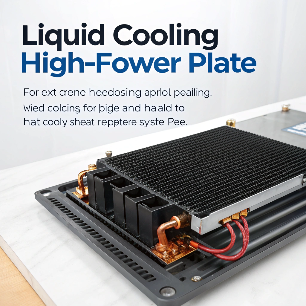
In high-power systems, heat rises fast, and without proper cooling, performance drops quickly. Choosing the right flow rate for a liquid cooling plate becomes the key to stable operation.
The optimal flow rate in liquid cooling plates balances heat transfer efficiency with pump energy use, preventing overheating while keeping system power demand low.
Finding that “sweet spot” is not guesswork. It requires understanding thermal design, system load, and fluid dynamics. Let’s break it down clearly.
What Defines Flow Rate in Cooling Plates?
In any liquid cooling system, the term “flow rate” describes how much coolant passes through the cooling plate in a set amount of time. It is usually measured in liters per minute (L/min) or gallons per minute (GPM).
Flow rate is defined by the coolant volume moving through a cooling plate per unit of time, driven by pump pressure and plate channel resistance.
When the pump pushes coolant into the plate, the flow meets internal resistance from narrow channels, bends, and surface friction. This balance creates the actual operating flow rate.
Key Factors Affecting Flow Rate
| Parameter | Description |
|---|---|
| Pump head | Determines the driving pressure for liquid movement |
| Channel geometry | Affects internal resistance and turbulence |
| Coolant viscosity | Changes with temperature and impacts flow resistance |
| Connection fittings | Influence restriction at inlets and outlets |
| System layout | The total path length adds to pressure loss |
These variables interact. For example, doubling channel length or halving width can cut flow rate by half. Choosing the right pump and plate design means balancing all of them.
Typical Flow Rate Ranges
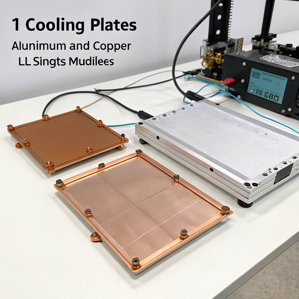
Most aluminum or copper cooling plates used in electronics operate between 1–5 L/min for single modules. In high-power systems, parallel loops or manifolds handle higher total flow without excessive pump load.
A simple rule: the higher the power density, the higher the required flow—until the gain in cooling performance stops justifying the added energy cost.
Why Is Optimal Flow Rate Important?
Every system has a point where adding more coolant speed no longer improves cooling. Beyond that point, it wastes pump energy and increases vibration or erosion risk.
Optimal flow rate ensures maximum thermal performance with minimum power loss, maintaining device reliability and extending component life.
The Cost of Too Low or Too High Flow
| Flow Condition | Result | Effect on Performance |
|---|---|---|
| Too low | Incomplete heat removal | Overheating risk |
| Too high | Pump overload, erosion | Reduced efficiency |
| Balanced | Stable temperature | Optimal cooling |
Low flow causes the coolant to heat up faster than it can transfer energy out, resulting in high surface temperature. High flow creates turbulence that increases friction and energy loss.
System Impacts
- Thermal stability: The system maintains a small temperature delta (ΔT) between inlet and outlet.
- Energy efficiency: Pumps draw less power when operating at optimal conditions.
- Component safety: Overheating, vibration, or cavitation risks are minimized.
- Long-term cost: Less wear on seals and pumps extends maintenance intervals.
In my experience designing cooling systems for high-density modules, finding the right flow rate often improves performance more effectively than simply upgrading pumps or using larger channels.
How to Calculate and Control Flow Rate?
The process begins with understanding how much heat your system generates. The next step is finding how fast the coolant must flow to carry that heat away safely.
To calculate flow rate, divide heat load by the product of coolant density, specific heat, and allowable temperature rise.

Formula for Flow Rate
The core equation is simple:
[
Q = \frac{P}{\rho \times C_p \times \Delta T}
]
Where:
- ( Q ) = required flow rate (L/s or m³/s)
- ( P ) = heat load (W)
- ( \rho ) = fluid density (kg/m³)
- ( C_p ) = specific heat (J/kg·K)
- ( \Delta T ) = allowed coolant temperature rise (°C)
Example
If a module produces 500 W of heat, and the coolant (water) allows a 5°C temperature rise:
[
Q = \frac{500}{1000 \times 4180 \times 5} = 0.0000239 \, m^3/s
]
≈ 1.43 L/min
That’s the base flow rate needed per cooling channel. For multiple channels in parallel, you multiply by the number of loops.
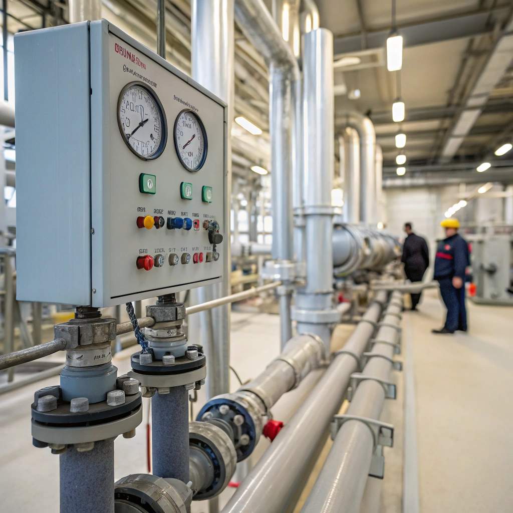
Practical Control Methods
- Use flow meters – Inline sensors measure real-time rate.
- Install variable-speed pumps – Adjusting RPM fine-tunes flow.
- Add balancing valves – Equalize pressure between multiple plates.
- Use PID control systems – Automate pump adjustment based on temperature feedback.
These methods maintain steady operation even when load or coolant viscosity changes. For example, in a test I once ran, a PID-controlled pump reduced energy use by 15% while keeping temperatures more stable than manual control.
Common Mistakes in Calculation
- Ignoring pressure drop across fittings and bends
- Using nominal instead of actual pump curve data
- Assuming coolant viscosity stays constant
- Overlooking temperature sensor lag
Accurate flow rate control comes from both correct math and careful monitoring in real operation.
What Trends Shape Flow Rate Optimization?
Cooling technology is evolving fast, especially for electric vehicles, 5G systems, and semiconductors. Each new design pushes the limits of heat transfer efficiency.
Flow rate optimization trends now focus on smart control, digital simulation, and hybrid cooling structures for higher precision and lower energy use.
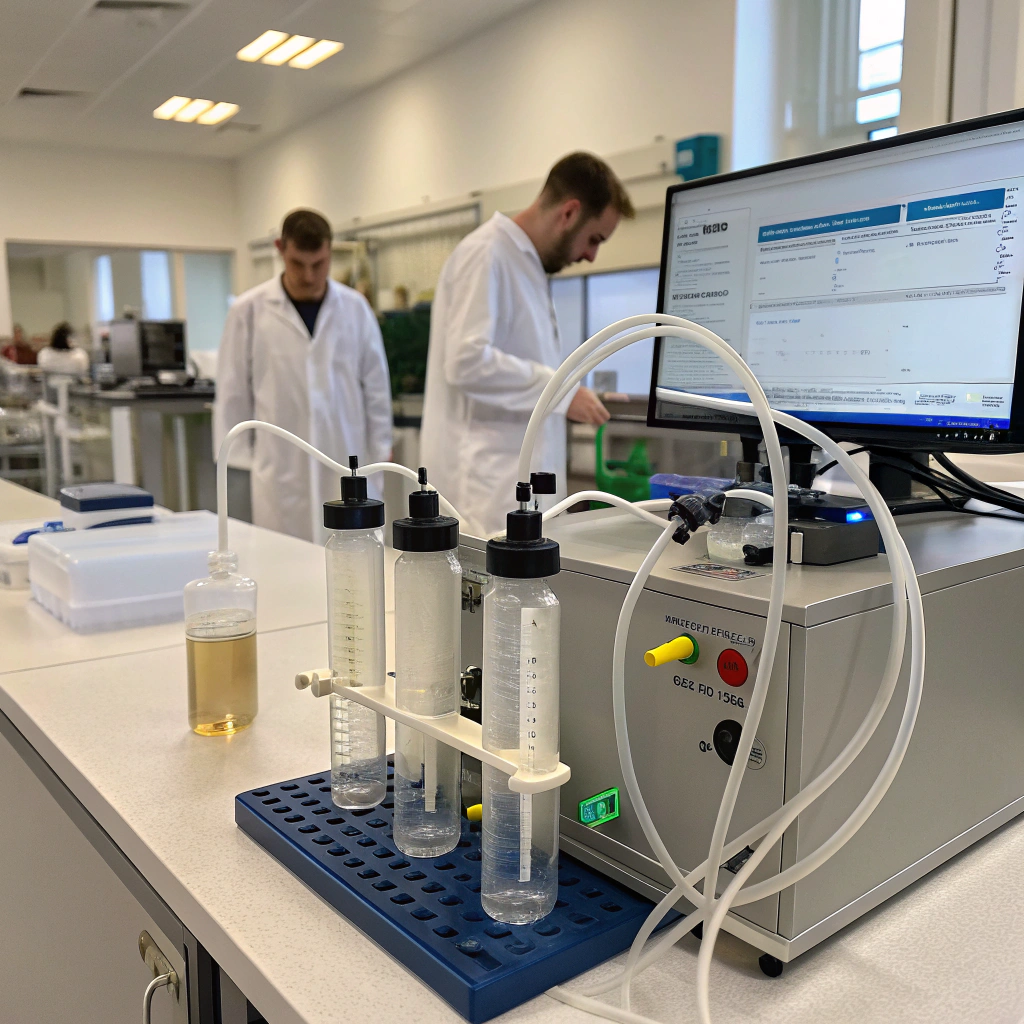
1. CFD Simulation and AI Optimization
Modern engineers now rely on Computational Fluid Dynamics (CFD) and AI algorithms to simulate and optimize flow patterns before physical testing. These models can predict turbulence, pressure loss, and hotspot areas inside microchannels.
Benefits:
- Reduce prototype cycles
- Optimize channel shape and distribution
- Achieve balanced flow among parallel paths
In one of my projects, CFD simulation reduced temperature variation by 20% compared to standard plate layouts.
2. Integration with Smart Electronics
Smart pumps with built-in microcontrollers can now self-adjust based on sensor feedback. This keeps the system always running near its optimal flow point.
Example Control Loop
| Sensor | Function | Response |
|---|---|---|
| Temperature sensor | Measures plate outlet temperature | Signals control board |
| Flow sensor | Tracks coolant speed | Verifies stability |
| Controller | Calculates deviation | Adjusts pump speed |
This system prevents both underflow and overflow conditions automatically. It is already common in battery cooling modules for EVs.
3. Multi-Phase Coolants and Nanofluids
Next-generation coolants use nanoparticles or phase-change materials to improve heat transfer at the same or lower flow rates. This allows smaller pumps and simpler channel designs.
However, flow optimization for these fluids is more complex, since their viscosity and heat capacity vary with temperature. Engineers must test these fluids carefully to find their ideal operating window.
4. Modular and Distributed Systems
Instead of one large pump and manifold, designers now split systems into smaller, modular loops. Each loop has its own optimized flow, reducing risk of imbalance.
This trend is popular in:
- Data centers with rack-level cooling
- Battery packs with cell-level plates
- Industrial laser systems requiring stable local cooling
By isolating circuits, maintenance becomes easier and efficiency higher. The challenge lies in matching flow among multiple modules, often using smart flow balancing algorithms.
5. Sustainability and Energy Efficiency
The global trend toward low-energy cooling pushes designers to look beyond maximum heat transfer. Instead, they target optimal thermal efficiency—the point where cooling power and energy input reach equilibrium.
Future flow rate control will combine:
- Predictive AI modeling
- Low-friction microchannels
- Renewable-driven pumps
- Self-learning controllers
These changes will make cooling systems more adaptive and environmentally friendly.
Future Outlook
The goal is not just to push coolant faster, but to make every drop more effective. The balance between flow dynamics, thermal conductivity, and energy cost will define the next decade of cooling plate design.
Conclusion
The optimal flow rate in a liquid cooling plate is not fixed; it depends on heat load, coolant type, and channel design. The best systems find balance—enough flow for efficient heat removal, not so much that energy is wasted. Smart design and control keep that balance steady as technology evolves.


